This blog post explores the fundamentals of the histogram and how to make it a valuable tool for analyzing image composition, leading to improved image quality and better imaging decisions for your specific image system application.
Histograms - The Basics
An image histogram groups pixel data by its intensity value and displays the quantity of each reported intensity value in the image. Using an example of an 8-bit image, the histogram would display a range of pixel values, from left to right, spanning from 0 [black] to 255 [white]. Simple images, such as pictures of black text on a white background will have relatively simple histograms with data only having a few values.
The following images showing simple geometric gray shapes on white backgrounds all have very simple histograms as the uniform shade of gray represents a single pixel intensity. Since the area (or combined area) of each shape is identical, the histograms of each image are identical.
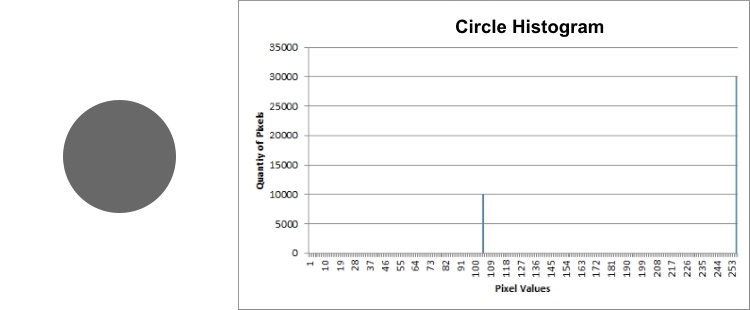

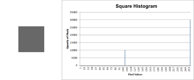
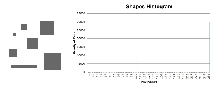
This illustrates that histogram data does not take into account the location of the pixels within the image. It simply shows the presence (or absence) of each possible pixel value. However, typical image histograms are much more complex than the two-tone sample images above.
Histograms and Bit Depth
The next image and associated histogram is representative of a typical 8-bit monochrome image.

Since the image consists of a large number of shades of gray, the histogram is distributed fairly evenly across all possible pixel values with a high spike at 255 due to the white background. This same image converted to 4-bit can be seen below with its associated histogram.
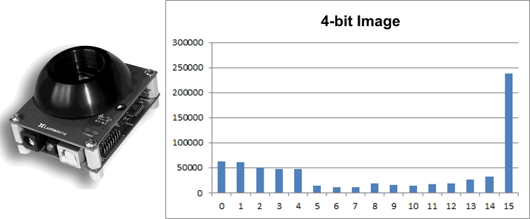
Here, the image shadows lack the smoothness that the 8-bit image has because there are only 16 values to transition from black to white. The histogram has the same general shape as the 8-bit image and has a large spike at 15 due to the white background. However, the scale on the y-axis is much larger since the same quantity of pixels is divided among 16 possible values instead of 255. The final image in this series shows a 1-bit image (either black or white) and its associated histogram.
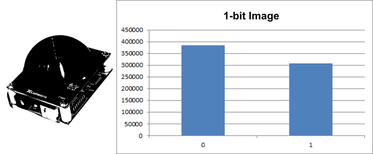
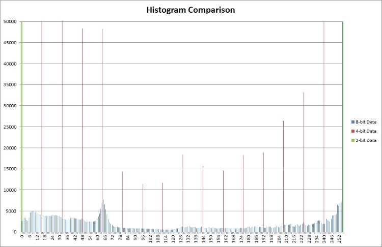
In this case, the image has very little detail because each pixel can only be either black or white. The histogram is trivial and shows the number of black and white pixels. The comparative histogram below shows how these three images would be represented on a span from 0-255.
Histograms and Exposure Time
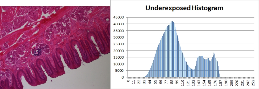
In the following series of images both the gain and gamma are set to 1.0. The first image is underexposed at 9ms. This can be seen by the lack of pixels with values above 195. Given the light background, the histogram should have values approaching the right edge of the graph.
Note: The images for the Histogram comparison below were captured with a Lumenera INFINITY-3-3URC microscope camera and microscope using a 10x objective, 0.63x coupler, daylight filter, and halogen lamp.
Increasing the image’s exposure will push the values to the right side of the histogram, indicating brighter pixels. The second image demonstrates an exposure time that is too long – 15ms, causing the image to be overexposed.
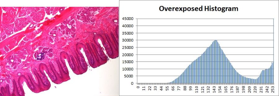
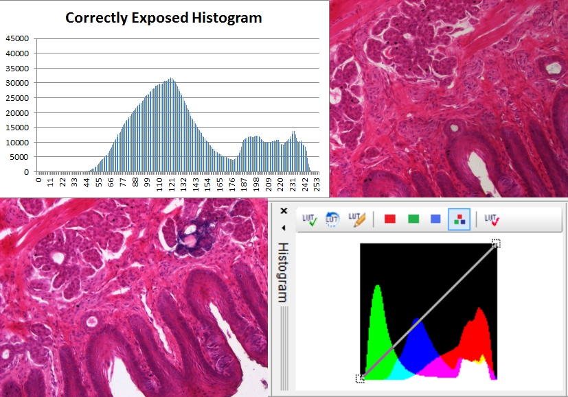
Here, the large spike to the right of the histogram indicates that the image is overexposed as data is being clipped or over saturated. A properly exposed image will have all available data contained within the histogram while making use of as many values as possible. The third and final image in this series illustrates a properly exposed image with an exposure time of 12ms.
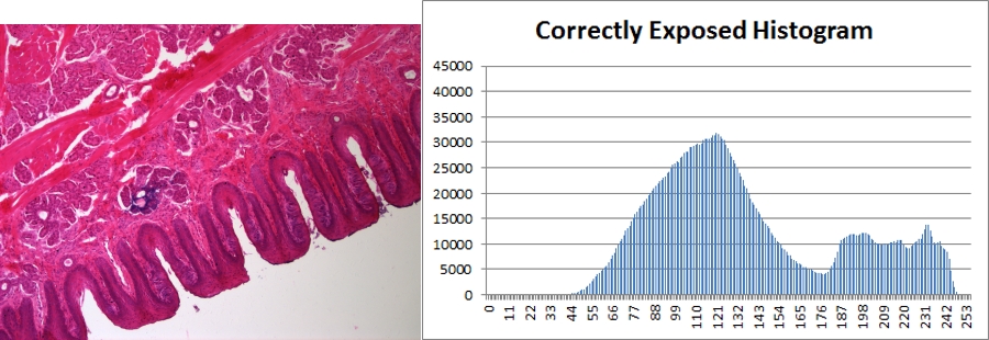
Note: Due to scaling and the lack of dark color in the image, the low number of dark pixels is not visible in the above histogram.
Here, the data is spread out widely across nearly the entire range of values supported by the camera at this bit depth. Since there is no black or dark color in the image, the left side of the histogram indicates that there are very few dark pixels. To the right, the values roll off just before saturation and ensure that no data is lost due to clipping. Comparing the underexposed and properly exposed histograms, it is obvious that the general pattern of the data is similar. In the properly exposed histogram, the camera settings are optimized to take advantage of the full range of values. In the overexposed histogram, the data is shifted too far into the bright area and results in a loss of data with pixels having a higher value.
Full Color Histograms
In the examples represented above, the grey-scale histograms reflect the average value for each pixel’s red, green, and blue values. They are histograms of the monochrome equivalent of each image. Histograms can represent each color channel that is present in a single image from a color camera and provide further information about the sensor’s response to the subject. Lumenera’s INFINITY ANALYZE software includes such histograms to provide the user with more comprehensive information regarding the color channel output. Below are the same three images as before, but with their color histograms.

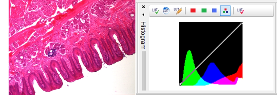
Starting again with the underexposed image, the image is lacking data to the right of the histogram. Additionally, you can see that the green channel is mostly dark since the colors of the image are stronger in the reds, purples, and magentas. The portion of the image that is simply a gray background with no specimen is illustrated by the portion of the histogram that is white. This highlights that all color channels are of equal value at that intensity level. Increasing the exposure to brighten this area, as in the next image, will fully saturate the pixels producing a white background.
The white portion of the histogram is pushed fully to the right, representing the now-white background of the image. Clipping can once again be observed – this time by the missing portion of the red channel. To have a properly exposed image, the histogram data for all three channels should be entirely contained within the histogram, as in the last image of the series below.
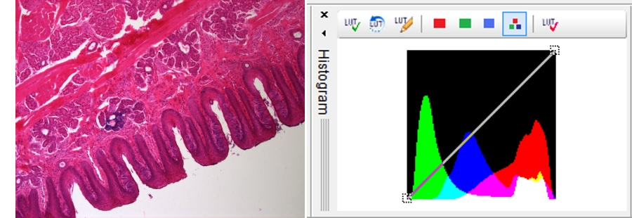
Here, all three color channels are contained within the histogram without being clipped by either edge. This translates into using the camera’s full dynamic range to expose the image. The very light gray background corresponds once again to the white portions of the histogram, in this case, pushed farther to the right indicating that the background is light, but not white since it is not touching the right edge.
Histograms provide useful information about the pixels intensity values that make up an image, especially around exposure accuracy and pointing out clipped data. When capturing an image while using a histogram, the main things to remember are to ensure data isn’t lost to clipping at either end of the histogram and to try and stretch the data across as much of the histogram as possible using settings such as exposure and analog gain to take advantage of the camera’s full dynamic range.
Learn More
To learn more, sign up for our newsletter to automatically receive regular updates from Lumenera.
