
Understanding the optical properties of your microscopy equipment will help you select the right digital camera for your microscope with the proper resolution for your specific application. Indeed, it is the properties of the microscope and not the camera that define the smallest resolvable detail in a slide.
As light travels through a small opening, it is subject to a phenomenon called diffraction. This is when light rays start to diverge from the incident axis and interfere with one another. The smaller the opening, the more pronounced the impact of diffraction. As the rays of light diverge, they travel different distances to their target – in this case, the camera’s image sensor.
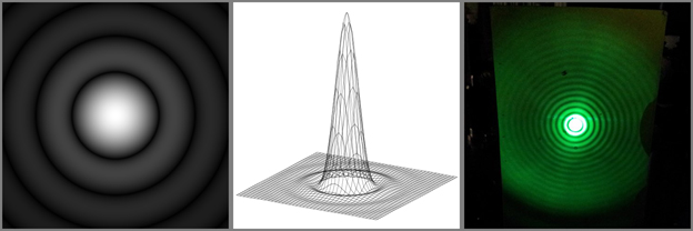
The change in distance traveled changes the phase of each ray of light, creating an interference pattern. If the small opening is circular, such as a microscope objective, the interference pattern that is created resembles a bull’s eye target and is known as an Airy disk. The below image demonstrates the Airy disk interference pattern. The left image is a simulated Airy disk pattern, the middle image is a 3D plot of the Airy disk’s intensity, and the right image is an actual Airy disk obtained by projecting a laser beam through a pinhole.
The optical system’s minimum resolution is directly tied to the size of the center circle of light and is defined by the diameter of the first dark circle. If the center circles of two Airy disks begin to overlap, a loss of sharpness will occur. If they overlap by more than the circles’ radius, they will no longer be resolvable. This is what is referred to as a diffraction limited system.
Below, the image on the left demonstrates two Airy disks that are fully resolvable, the center image shows Airy disks that are at the critical overlap point, and the right image shows two Airy disks that are no longer resolvable.

The two variables that dictate the size of the Airy disk in a microscope are the objective’s numerical aperture (NA) and the wavelength of light (λ) used. We can use the Rayleigh criterion to determine the smallest resolvable dimension by an optical system using these variables in the equation below:

In the case of a 20x objective with an NA of 0.5, using green light (λ = 550nm), the smallest resolvable dimension is 0.671µm. This dimension is magnified by the product of the objective and coupler magnifications when projected onto the image sensor. In the case of a 0.5x coupler, commonly paired with a 1/2" sensor, and the 20x objective, this dimension becomes 6.71µm. To properly sample this dimension, the Nyquist theorem requires a pixel size of at least half of this smallest resolvable dimension. Therefore the camera’s image sensor should have pixels no larger than 3.36µm each to correctly resolve this dimension at this magnification.
By modifying the values of certain variables, we notice that a larger NA will require smaller pixels for the same magnification since there is less diffraction. Conversely, if red light is used, the pixels can be larger because the wavelength of the light is longer. An increase in magnification will also allow for larger pixels as the minimum resolvable dimension is projected onto a larger area of the sensor. Because the minimum resolvable dimension of objects increases when enlarged with higher magnification (eg: 60X or 100X), using smaller pixels will not add any additional detail as no additional information exists. Larger pixels will adequately collect all of the available detail in a highly magnified image, and therefore a lower resolution sensor (for a given sensor format size) is all that’s required. Given that light is being collected from a smaller area of the slide at higher magnifications, the larger pixels will also contribute towards increased sensitivity of the camera. This lends itself well to other applications where low light is an issue and high sensitivity is required.
The table below gives a few concrete examples with various objective magnifications and numerical apertures. It is important to note that even though the Nyquist theorem requires the minimum resolution to be halved to determine the pixel size, monochrome sensors will better resolve small dimensions if the minimum dimension is divided by three; and by four for color sensors, due to the layout of the Bayer filter pattern on the pixels. The table below illustrates the largest possible pixel size required to fully resolve the smallest visible detail of an object using the wavelength, coupler, and sensor size from the previous example: 550nm, 0.5x, and 1/2", respectively.
| Magnification / NA | Resolution Limit (µm) | Projected Size (µm) | Required Pixel Size (µm) Mono / Color | Sensor Resolution (Mono) |
|---|---|---|---|---|
| 10x / 0.30 | 1.12 | 11.2 | 3.73 / 2.80 | 1717 x 1288 |
| 20x / 0.50 | 0.67 | 13.4 | 4.47 / 3.36 | 1431 x 1073 |
| 40x / 0.75 | 0.45 | 17.9 | 5.96 / 4.47 | 1073 x 805 |
| 60x / 0.85 | 0.39 | 23.7 | 7.89 / 5.92 | 811 x 608 |
| 100x / 1.30 | 0.26 | 25.8 | 8.60 / 6.45 | 744 x 558 |
Why not select a camera with the smallest pixel size possible? Because large pixels collect more light. This means there is a trade-off between resolution and sensitivity and a balance between these two factors will provide the optimal solution. The pixels should be small enough to resolve the necessary amount of detail yet large enough to capture a sufficient amount of light to generate a quality image, without requiring long exposure times.
If you’re debating between two cameras with identical sensor sizes and differing sizes of pixels, err on the side of smaller pixels. Generally speaking, image sensors with more pixels will have smaller pixels. As such, the sensor will give you more resolution at a cost of less sensitivity. However, Lumenera CCD cameras support a feature known as “pixel binning”, where the software will group a cluster of pixels together to form a larger “super pixel”.
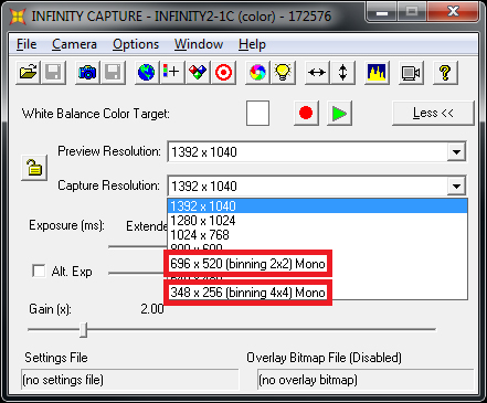
This will help increase the sensor’s sensitivity and can be used in scenarios such as imaging at higher magnifications, where high pixel density isn’t required and larger pixels are preferred for increased sensitivity.
